Abstract

The Attention Mechanism is a flexible and powerful framework. However, it might be super confusing because of its flexibility. This article explains the concept of Query, Key, Value, and Output with an analogy of an Information Retrieval System. This article also shows how to achieve different Attention Mechanisms by varying:

1. Query-Key compatibility function
2. Query, Key, and Value choices

For example, the innovation of Self-Attention is to use the same vector as Query, Key, and Value, while the innovation of Scaled Dot-Product Attention is to have a different Query-Key compatibility function.

Information Retrieval System

An Information Retrieval System stores Values indexed by Keys. A Query is used to retrieve related Key-Value pairs. The system returns an Output that is the associated Value or a transformed version of the associated Value.

Exact Matching

Fig.1 Finding the Exact Income by a Person's Name

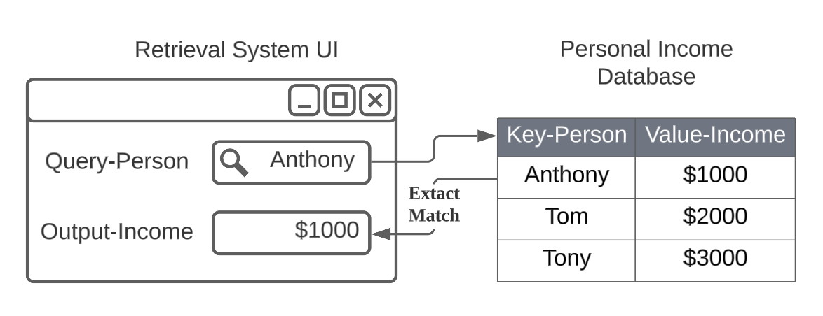
In Fig.1, we have a basic system that allows users to find the exact income by a person's name. The system stores the Values (Income) indexed by Keys (Name). When a user enters a Query (Name), the system returns an Output (Income) where it is the Value (Income) that is related to the Query (Name).

Query-Key Compatibility

Fig.2 Estimating a Person's Income by His/Her Name

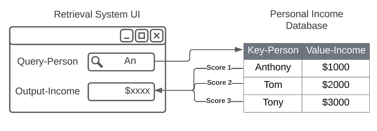
Sometimes, we might not want an exact matching between Query and Key. For example, in Fig.2, we want to estimate a person's income by their name. The Query might not be the same as the Key (Name). In this case, the system computes Query-Key compatibility scores between the Query and all the Keys (Name) in the system.

We can use different functions to measure compatibility. The compatibility function takes the Query and Key as inputs and gives a score.

Note: Query-Key compatibility has also been called similarity, relevancy, and alignment in different places.

Retrieval Output - Weighted Sum of Values

The returned Output is the weighted sum of all Values, which is weighted by the Query-Key compatibility scores.

For example, in Fig.2,

1. If the scores are $[0.9, 0.1, 0.0]$ respectively, the returned Output will be $1000 \times 0.9 + 2000 \times 0.1 + 3000 \times 0.0 = 1100$.

2. If the scores are $[1.0, 0.0, 0.0]$ respectively, the returned Output will be $1000$, the same as retrieving the Value with the highest associated compatibility score.

Information Retrieval in Sequential Data

We have discussed the Query-Key compatibility in terms of an Information Retrieval System, but how can we apply it to Deep Learning? We can use different Queries, Keys, and Values choices for various NLP tasks. Let's consider a simple task below:

For a 5-word sentence: "i like to eat apple", we want to know if the word "apple" is a fruit or a company.

Let's have the following Queries, Keys, and Values choices:

• Keys = Values as five embedding vectors of each word = $\mathbf{k}_{1 \le s \le 5}$
• Query as the embedding vector of the word "apple" = $\mathbf{q}$

Note: This configuration is the same as the Self-Attention (Will be discussed below).

To understand if the word "apple" is a fruit or a company, we need to know the context of the sentence. We can compute compatibility scores to determine which words we should focus on to decide if the word "apple" is a fruit or a company.

Ideally, we want the Key "eat" to have a higher score than the other Keys when Query is "apple", for example $(\mathbf{q}, \mathbf{k}_4)$ should be more compatible than $(\mathbf{q}, \mathbf{k}_3)$.

Let's make up some scores such that only the Keys "eat" and "apple" have a high score with the Query "apple":

Then the Output for the Query "apple" will be the weighted sum of all Values:

The General Form of Attention Mechanism

An attention function can be described as mapping a query and a set of key-value pairs to an output, where the query, keys, values, and output are all vectors. The output is computed as a weighted sum of the values, where the weight assigned to each value is computed by a compatibility function of the query with the corresponding key. -- Attention Is All You Need¹

Query, Key, Value, and Output Vectors

In the setting of deep learning, we have a Query vector $\mathbf{q}$, a Key vector $\mathbf{k}$, and a Value vector $\mathbf{v}$. They are in their own spaces, that's $\mathbf{q} \in \R^{d_q}$, $\mathbf{k} \in \R^{d_k}$ and $\mathbf{v} \in \R^{d_v}$. The returned output vector $\mathbf{o}$ is in the Value space, that's $\mathbf{o} \in \R^{d_v}$.

Recall the Key-Value setting for Sequential Data above; let's say there is a sentence with length $S$, then there will be $S$ Key vectors and $S$ Value vectors. We can represent them as two matrices:

Query-key Compatibility Function

A Query-Key compatibility function $f_{\mathbf{compatibility}}: (\R^{d_q}, \R^{d_k}) \to \R$ maps a Query vector and a Key vector to a score scalar. The higher the score, the more compatible the Query vector and Key vector are. We will have $S$ compatibility scores:

Attention Weights and the Output Vectors

The attention weights are usually defined by applying softmax to the compatibility scores, such that the sum of the weights is 1. The softmax function is defined as:

Here is how we compute these $S$ attention weights:

Then the Output vector $\mathbf{o} \in \R^{d_v}$ is the weighted sum of those $S$ Value vectors:

In matrix form, given $\mathbf{Q} \in \R^{T \times d_q}$, $\mathbf{K} \in \R^{S \times d_k}$, $\mathbf{V} \in \R^{S \times d_v}$, and a compatibility score matrix $\mathbf{E} \in \R^{T \times S}$:

Different Query-Key Compatibility Functions

Dot-Product Attention

Regarding the angular similarity between two vectors, Dot-Product is a common choice. Dot-Product Attention refers to having the compatibility function as the dot-product of the Query vector and Key vector. ²

In matrix form, given $\mathbf{Q} \in \R^{T \times d_k}$ and $\mathbf{K} \in \R^{S \times d_k}$, $\mathbf{V} \in \R^{S \times d_v}$:

Dot-Product Attention is the simplest compatibility measure form, as there are no hidden learning weights in the compatibility function. However, this method assumes both Query and Key vectors have the same dimension.

Scaled Dot-Product Attention

Scaled Dot-Product Attention is a variant of Dot-Product Attention, where we scale the dot-product by a factor $\frac{1}{\sqrt{d_k}}$. ³

In matrix form, given $\mathbf{Q} \in \R^{T \times d_k}$ and $\mathbf{K} \in \R^{S \times d_k}$, $\mathbf{V} \in \R^{S \times d_v}$:

This is the form shown in the original Transformer paper ³.

Query, Key, and Value Linear Transformation

Fig.3 Linear Transformation Before Dot-Product in Transformer

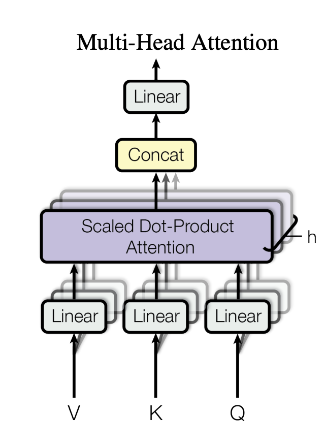
Note: In Fig.3 and the original Transformer paper, the labels "Q", "K", "V" at the bottom refer to the input to the linear layers (before projection). The actual Query, Key, Value vectors used in the attention computation are the outputs of these linear layers (after projection).

In practice, the input to an attention layer is a matrix $\mathbf{X} \in \R^{S \times d_{\text{model}}}$. The model projects $\mathbf{X}$ into Query, Key, and Value matrices using three learnable weight matrices:

where $\mathbf{W}_Q \in \R^{d_{\text{model}} \times d_k}$, $\mathbf{W}_K \in \R^{d_{\text{model}} \times d_k}$, and $\mathbf{W}_V \in \R^{d_{\text{model}} \times d_v}$.

These projection matrices $\mathbf{W}_Q$, $\mathbf{W}_K$, $\mathbf{W}_V$ are the only learnable parameters in the attention mechanism. The compatibility function itself (e.g., dot-product) has no learnable weights — all learning happens through these projections.

Substituting into the Scaled Dot-Product Attention formula, we get the full equation:

Different Query, Key, Value Choices

Other than varying the Query-Key compatibility function, we can also change the Query, Key, and Value choices. We can combine different compatibility functions and Query, Key, and Value choices to construct other attention mechanisms. ⁴

For example, in Transformer, we have Self-Attention with Scaled Dot-Product Compatibility Function.

Fig.4 Different Attention Layers in Transformer

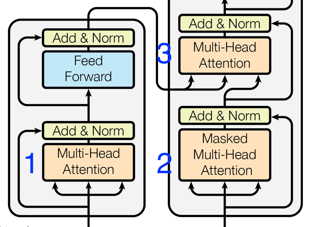
We can examine different Query, Key, and Value choices in the standard Transformer model in Fig.4.

Self-Attention [Fig.4 - 1, 2]

When we have the same Query vectors, Key vectors, and Value vectors, we call it self-attention. The example stated in the "Information Retrieval in Sequential Data" section above is a self-attention example.

Self-Attention has the following choices:

• Keys = Values are embedding vectors of each word in a sequence = $\mathbf{k}_{1 \le s \le S}$
• Query is an embedding vector of a word in the same sequence = $\mathbf{q}_{1 \le s \le S}$

The masked self-attention is a variant of self-attention where we mask the attention weights of the future words. This is used in the Transformer decoder to prevent positions from attending to subsequent positions.