Overview

Machine Learning Refresher is a series of articles that records my journey of relearning the fundamentals of Machine Learning.

This article is a compiled version of

• Section 1.2 Probability Theory of the "Pattern Recognition and Machine Learning" book.
• MSBD5012 Machine Learning course materials
• Other online resources
• My own understandings

I added two things here to enhance my understanding:

• Emphasis on probability vs. probability distribution.
• Python code to generate an example.

Sample Space and Event of a Random Experiment

A Random Experiment is a process with uncertain outcomes. A set of all the possible outcomes of the random experiment is called the Sample Space $\Omega$.

• If rolling one dice is the random experiment, the sample space $\Omega = \{1, 2, 3, 4, 5, 6\}$.

A Random Variable is a function that takes a sample space and maps it to a new sample space:

• The easiest one is the identical (1-to-1) function, let the Random Variable $X$ be the outcomes (the sample space) of rolling one dice (the random experiment). $X$ takes values $\Omega_{X} = \{1, 2, 3, 4, 5, 6\}$, as well.

A Event is a subset of a sample space $\Omega$:

• $(X=2)$ describes an Event subset $\Omega_{X=2}=\{2\}$, and it describes we got a value $2$ from the random experiment of rolling one dice.
• $(X=\mathbf{Odd})$ describes an Event subset $\Omega_{X=\mathbf{Odd}}=\{1, 3, 5\}$, and it describes we got a odd number value from the random experiment of rolling one dice.

A Composed Experiment describes the repetitions of the same random experiment, and each repetition can be called a trail.

Probability and Probability Distribution

Let's consider a random variable $X$ with $M$ discrete outcomes $\Omega_{X}=\{x_1, x_2,..., x_i, ... x_M\}$.

$P(X=x_i)$ denotes the probability of an event of $X$ being $x_i$. For example, if $X$ is the smartphone model we found in a random experiment, $P(X=\mathbf{IPhoneSE})$ is the probability of finding an IPhoneSE smartphone in the random experiment.

Taking all outcomes into account, $P(X)$ denotes the probability distribution of $X$:

• Probability Mass Function (Histogram) for discrete outcomes.
• Probability Density Function for continuous outcomes.

Joint Probability

Let's say there are two random variables $(X, Y)$ in a random experiment.

• $X$ has M outcomes $\Omega_{X} =\{x_1, x_2, ..., x_i, ..., x_M\}$.
• $Y$ has L outcomes $\Omega_{Y} =\{y_1, y_2, ..., y_j, ..., y_L\}$.

Then each observation in the random experiment is a pair of events $(X=x_i, Y=y_j)$. $P(X=x_i, Y=y_j)$ denotes the joint probability of two events, $(X=x_i)$ and $(Y=y_j)$, occurring at the same time.

For example, if $X$ and $Y$ are the smartphone model and the gender we found in an random experiment, respectively, $P(X=\mathbf{IPhoneSE}, Y=\mathbf{Male})$ indicates the probability of finding a male with IPhone SE in the random experiment.

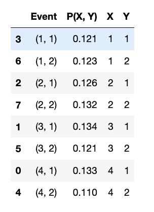
After obtaining the joint probability of each $(X=x_i, Y=y_j)$ pair, we can get the joint probability distribution $P(X, Y)$. To illustrate this idea, the following code generates 1000 $(X=x_i, Y=y_j)$ pairs (xs and ys):

# Take 1000 samples between [1, 5)
xs = [np.random.randint(1, 5) for _ in range(1000)]
# Take 1000 samples between [1, 3)
ys = [np.random.randint(1, 3) for _ in range(1000)]
# Count the (x, y) pairs and convert them to a dataframe
joint_dist_df = pd.DataFrame.from_dict(Counter(zip(xs, ys)), orient="index").reset_index()
joint_dist_df.columns = ["Event", "P(X, Y)"]
joint_dist_df["X"] = [e[0] for e in joint_dist_df["Event"]]
joint_dist_df["Y"] = [e[1] for e in joint_dist_df["Event"]]
# Compute the joint probability
joint_dist_df["P(X, Y)"] /= joint_dist_df["P(X, Y)"].sum()
joint_dist_df

The above code generates the following dataframe:

Joint Probability Distribution $P(X,Y)$

Marginal Probability

Based on the observations of $(X=x_i, Y=y_j)$ we can calculate the marginal probability $P(X=x_i)$ by marginalizing $Y$:

For example, if $X$ and $Y$ are the smartphone model and the gender we found in a random experiment, respectively. We can compute $P(X=\mathbf{IPhoneSE})$ by adding up the corresponding joint probabilites for each gender.

Applying this to all $X$'s outcomes we get the marginal probability distribution $P(X)$:

This is called the sum rule of probability theory. The following code shows how to compute the marginal probability distribution:

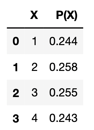
marginal_x_dist_df = joint_dist_df.groupby("X")["P(X, Y)"].sum().reset_index()
marginal_x_dist_df.columns = ["X", "P(X)"]
marginal_x_dist_df

The above code generates the following dataframe:

Marginal Probability Distribution $P(X)$

Conditional Probability

If we filter the observations by a particular outcome (e.g., $X=x_i$), we can calculate the probabilities of observing $Y=y_j$ given the filtered observations $(X=x_i)$. It is called the conditional probability $P(Y=y_j|X=x_i)$

The following code shows how to compute the conditional probability distribution $P(Y|X)$:

for x_i in range(1, 5):
    print("For x_i =", x_i)
    # Filter obseravtions based on x_i
    _df = joint_dist_df[joint_dist_df["X"]==x_i].copy()
    _df = pd.merge(_df, marginal_x_dist_df, how="left", on="X")
    # Calculate the conditional probabilites
    _sum = _df["P(X, Y)"].sum()
    _df["P(Y|X)"] = _df["P(X, Y)"] / _sum
    display(_df)

The above code generates the following dataframe:

Conditional Probability Distribution $P(Y|X)$

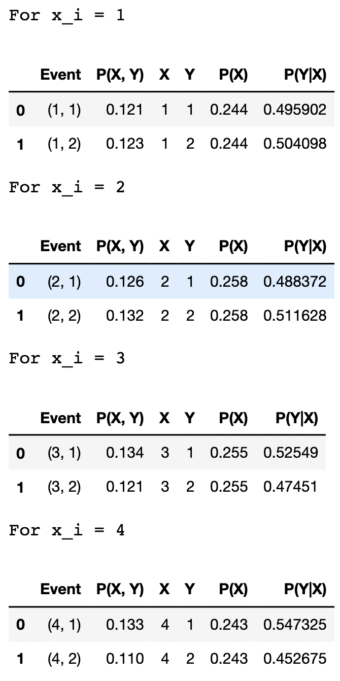
From the result we can also observe that the conditional probability $P(Y=y_j|X=x_j)$ can be calculated with:

And the conditional probability distribution can be written as:

And, $P(X,Y)=P(Y|X)P(X)$ is called the product rule of probability theory.

Independence

There is a special case for the product rule above. If two events $X=x_i$ and $Y=y_j$ are independent, Knowing $X=x_i$ in advance won't change the probability of having $Y=y_j$; therefore:

• The conditional probability becomes $P(Y=y_j|X=x_i) = P(Y=y_j)$
• The conditional probability distribution becomes $P(Y|X) = P(Y)$

Applying this new information to the product rule above we will get:

if $X=x_i$ and $Y=y_j$ are independent.

Test of Independence

# Take 1000 samples between [1, 5)
xs = [np.random.randint(1, 5) for _ in range(1000)]
# Take 1000 samples between [1, 3)
ys = [np.random.randint(1, 3) for _ in range(1000)]

In the Python coding example, we generated 1000 $(X=x_i, Y=y_j)$ pairs (xs and ys) uniformly and independently. But why we are not getting a perfect result of $P(X, Y) = P(X) \times P(Y)$?

We can find the root cause by looking at the marginal probabilities of $X$ and $Y$. Ideally we should see $P(X=x_i)=0.25$ and $P(Y=y_j)=0.5$, but it is not the case.

We can use the Chi-squared test to test if two categorical values are independent.

Chi-squared test tests if two categorical variables are dependent on each other or not.

• The null hypothesis: $(X=x_i)$ and $(Y=y_j)$ are independent.
• The alternative hypothesis: $(X=x_i)$ and $(Y=y_j)$ are dependent.

from sklearn.feature_selection import chi2
# The null hypothesis is that they are independent.
# P <= 0.05: Reject the null hypothesis.
# P > 0.05: Accept the null hypothesis.
chi2(np.array(xs).reshape(-1, 1), np.array(ys).reshape(-1, 1))
# > (array([0.88852322]), array([0.34587782]))

The test returns a P-value of 0.346; therefore, we cannot reject the null hypothesis that $(X=x_i)$ and $(Y=y_j)$ are independent. So there is a problem in the process above: the probabilities obtained from counting observations are not entirely accurate.

Frequentist Probability and Bayesian Probability

The entire discussion above is based on counting observations. It is called the Frequentist Probability. The Frequentist Probability requires many repetitions of a random experiment to have an accurate probability distribution. In the code example, we only sampled 1000 $(X=x_i, Y=y_j)$ pairs (xs and ys), which is too small. If we increase the sample size, we can see the marginal probabilities will get closer to the ideal values.

However, it is hard to produce the exact $P(X, Y) = P(X) \times P(Y)$ even with a very large number of trials. In this case, since we know xs and ys are generated from two independent processes, we can set $P(X=x_i)=0.25$ and $P(Y=y_j)=0.5$ manually instead. This is a perspective of Bayesian Probability. In Bayes' Theorem, $P(Y=y_i)$ is the prior probability, which is set by humans.

In other words, based on the human knowledge, we can decide if we want to use the $P(X)$, $P(Y)$ from counting observations or use the following theorical values:

• Set $P(X)$ to be a uniform distribution with $P(X=x_i)=0.25$
• Set $P(Y)$ to be a uniform distribution with $P(Y=y_j)=0.5$

In general, prior probability (human knowledge) is better for a small dataset because Frequentist Probability requires a large dataset. However, one clear disadvantage of Bayesian Probability is that based on personal belief, it could be wrong that I assumed xs and ys come from two independent processes. A bad prior probability distribution setup is a problem for Bayesian Probability.

Bayes' theorem

Recall the product rule $P(X=x_i,Y=y_j)=P(Y=y_j|X=x_i)P(X=x_i)$, since joint probability distribution is symmetrical $P(X=x_i,Y=y_j) = P(Y=y_j,X=x_i)$, we can deduce the Bayes' theorem like this:

• $(Y=y_j)$ is the event we want to analyze and $(X=x_i)$ is the event we takes as an evidence to support the occurance of $(Y=y_j)$.
• $P(Y=y_j)$ is the prior probability of $(Y=y_j)$ without knowing $(X=x_i)$ as an evidence. It is the best guess of the probability of $(Y=y_j)$ occurring without new information.
• $P(X=x_i)$ is the prior probability of finding the evidence. It normalize the likelihood $P(X=x_i|Y=y_j)$.
• $P(X=x_i|Y=y_j)$ is the likelihood. it can be written as $L(Y=y_j|X=x_i)$.It is the probability of finding the evidence $(X=x_i)$ given the $(Y=y_j)$ has already occured.
• $P(Y=y_j|X=x_i)$ is the posterior probability we want to calculate after seeing an evidence $(X=x_i)$.

In-terms of probability, $P(Y=y_j|X=x_i)$ describes the probability of finding our target $(Y=y_j)$ given the evidence $(X=x_i)$. $P(Y=y_j)$ describes the probability of finding our target $(Y=y_j)$ before knowing the evidence $(X=x_i)$. If the new evidence $(X=x_i)$ is value-adding, we should see $P(Y=y_j|X=x_i)$ deviates from $P(Y=y_j)$. In other words, the new evidence $(X=x_i)$ can update our degree of belief $P(Y=y_j)$.

Therefore, $\frac{P(X=x_i|Y=y_j)}{P(X=x_i)}$ can be understood as the support of the evidence for our target, since $\frac{P(X=x_i|Y=y_j)}{P(X=x_i)} > 1 \rightarrow P(Y=y_j|X=x_i) > P(Y=y_j)$, . This shows the evidence $(X=x_i)$ is for $(Y=y_j)$.

TODOs:

• Example for Bayesian update.
• Dive deeper into Bayesian inference.

Estimating a Model's Parameter

TODO