Overview

This was a 1-month competition¹ hosted by the Eterna community and Stanford DasLab on Kaggle. In the competition, we were given a set of mRNA sequences and their corresponding likelihood of degradations at the base/linkage after incubating with magnesium, high pH, or high temperature.

The code is released on Github.

The original short write-up on Kaggle.

Problem Statement

Fig.1 mRNA Degradation¹

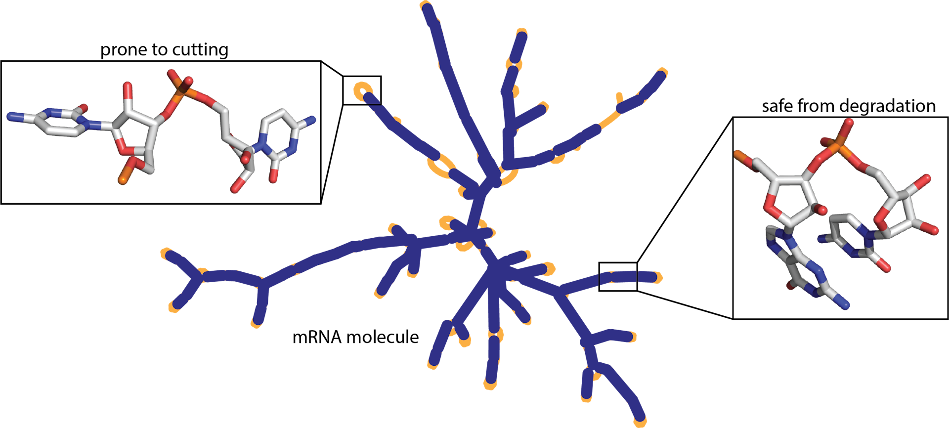
One of the biggest problems of mRNA vaccines is its tendency to degrade spontaneously. If an mRNA vaccine degrades, it becomes useless. Therefore, the mRNA vaccines must be prepared and shipped under intense refrigeration. This becomes a significant barrier in delivering mRNA vaccines to areas lacking proper logistical and medical infrastructure.

In the competition, we were asked to predict the degradation rates at each base of an RNA molecule given a subset of an Eterna dataset comprising over 3000 RNA molecules (which span a panoply of sequences and structures) and their degradation rates at each position.

Data Description

Feature: mRNA Sequence

Messenger RNA (mRNA) sequence is represented as a string in the dataset like this: GGAAAAGCUCUAAUAACA...

There are 4 bases in a mRNA sequence: adenine (A), thymine (T), guanine (G) or cytosine (C). 3 bases form a group (codon); therefore it is like 3-gram in NLP.

mRNA sequences data have 107 bases and 130 bases in the training and validation sets, respectively.

Feature: Predicted mRNA Structure & Loop Type

A mRNA sequence can have different structures. In this competition, we were given 2 features: structure and predicted_loop_type. They describe the secondary structure of a mRNA sequence predicted by Vienna RNAfold 2².

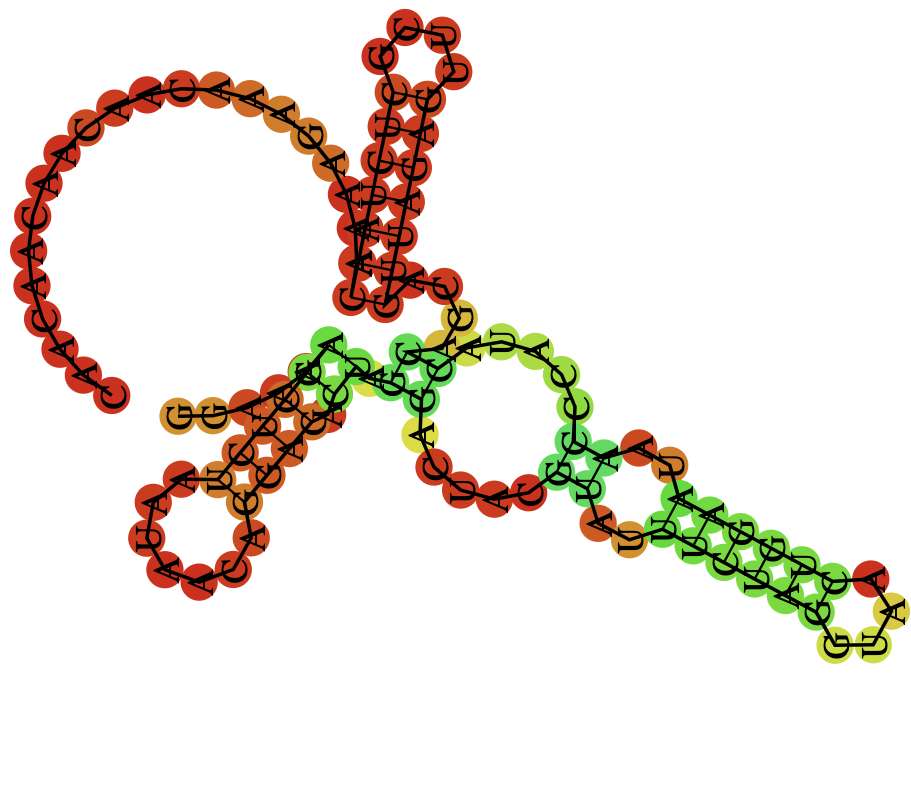
Fig.2 RNAfold Result³, a darker color indicates a higher base pairing probability

The result shown in Fig.2 is the RNAfold result of the following mRNA sequence. The corresponding structure and predicted_loop_type are represented as strings in the dataset:

Fig.3 RNAfold Result String Representation¹

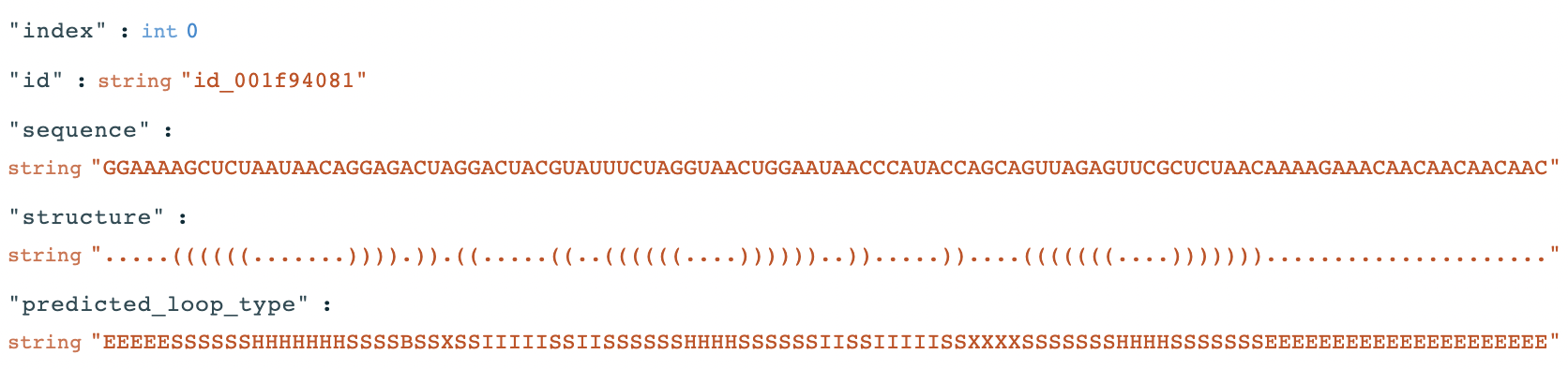
Paired bases are denoted by opening and closing parentheses in the structure field. Loop types are coded by -- S: paired "Stem", M: Multiloop, I: Internal loop, B: Bulge, H: Hairpin loop, E: dangling End, and X: eXternal loop in the predicted_loop_type field.

Feature: Base Pairing Probabilities

The Base Pairing Probabilities is a (107 x 107 or 130 x 130) matrix that describes the probability of 2 positions of an mRNA sequence being paired ⁴. The visualization can be seen in Fig.2 above.

Targets

Only 68 bases were labeled in an mRNA sequence in the training data, while in the test set, 91 bases were labeled. Therefore, the model has to be trained on a shorter sequence and inference on a longer sequence. There are 5 targets for each base:

reactivity: The reactivity values of each base of an mRNA sequence. It is used to determine the likely secondary structure.

deg_pH10: The reactivity values of each base of an mRNA sequence that's used to determine the likelihood of degradation at the base/linkage after incubating without magnesium at high pH (pH 10).

deg_Mg_pH10: The reactivity values of each base of an mRNA sequence that's used to determine the likelihood of degradation at the base/linkage after incubating with magnesium in high pH (pH 10).

deg_50C: The reactivity values of each base of an mRNA sequence that's used to determine the likelihood of degradation at the base/linkage after incubating without magnesium at high temperature (50 degrees Celsius).

deg_Mg_50C: The reactivity values of each base of an mRNA sequence that's used to determine the likelihood of degradation at the base/linkage after incubating with magnesium at high temperature (50 degrees Celsius).

Evaluation

The evaluation was done via the MCRMSE (mean column-wise root mean squared error) metric. In the test set, only three targets (reactivity, deg_Mg_pH10, and deg_Mg_50C) are scored.

Where

• $N_t$ denotes the number of scored targets (5 in train and 3 in test)
• $n$ denotes the number of required & scored bases (68 in train and 91 in test)
• $y_{ij}$ and $\hat{y}_{ij}$ denote the prediction and the ground truth for each $i$-th base and $j$-th target column, respectively.

Methodology

Architecture Overview

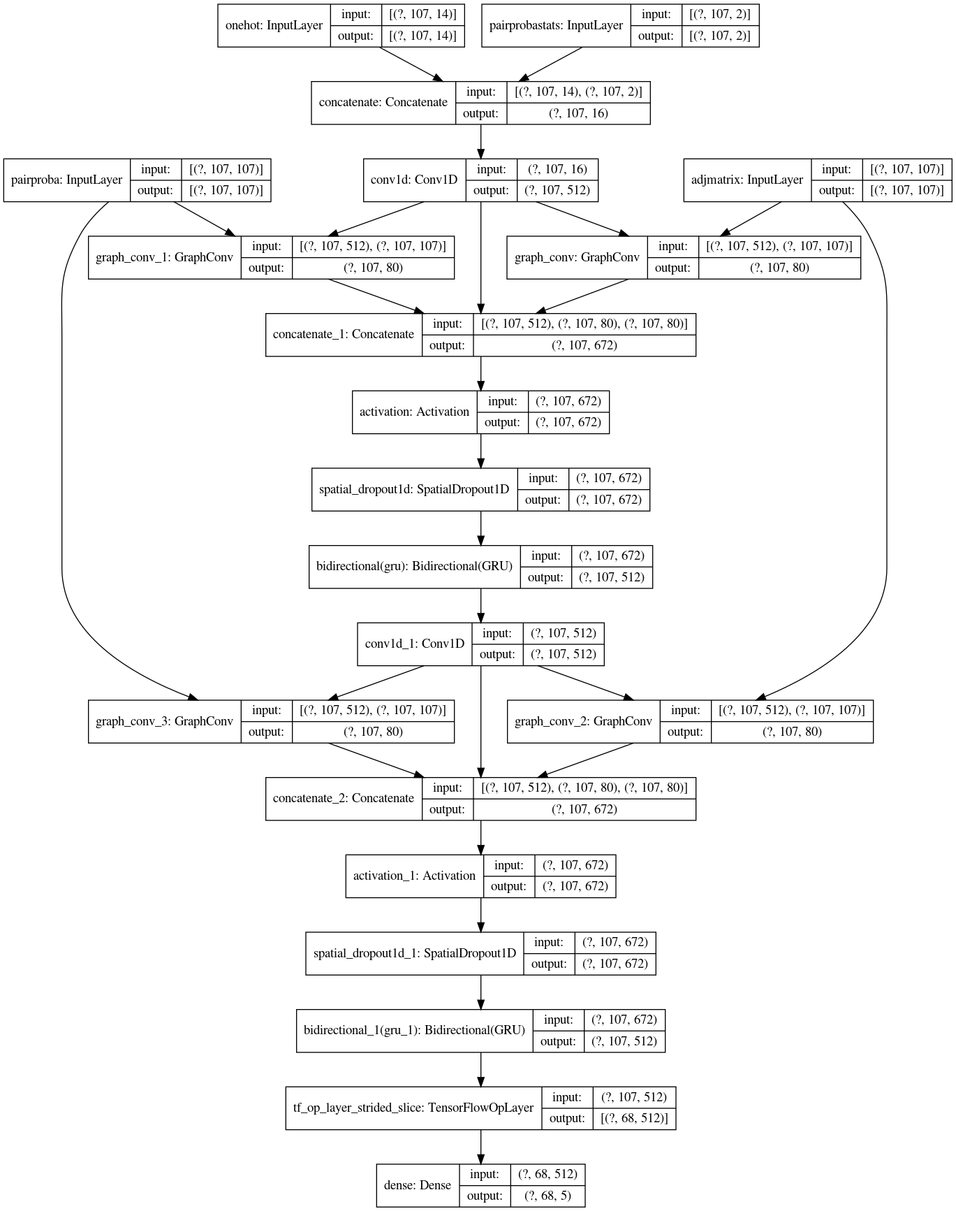
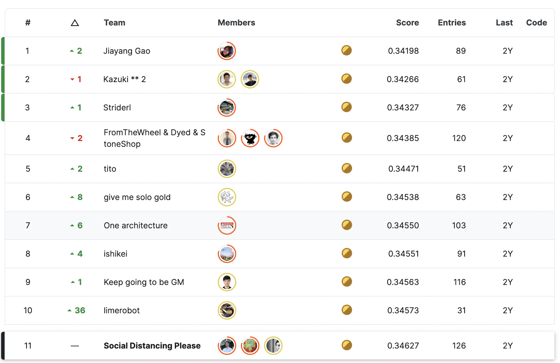
Our 11-th place solution is an ensemble of multiple models. There are mainly two types of models. The first type is a combination of 1D Convolution Layers, Graph Convolution Layers, and RNN Layers. The second type is a combination of WaveNet layers and RNN Layers. The most powerful features are the adjacency matrices constructed by the given structure sequence and base-pair probabilities. The adjacency matrices are used for the Graph Convolution Layers.

My work was mainly on the first type of model (1D Convolution Layers, Graph Convolution Layers, and RNN Layers). The model summary of a simplified version is reported in Fig.4.

Fig.4 Simplified model summary⁵

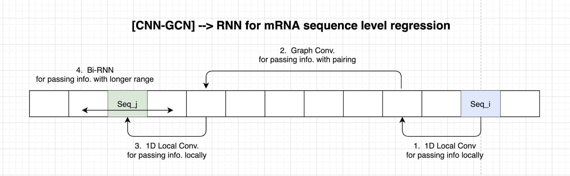
Ideation

At first, most of the Kaggle teams were using only RNN models. There were discussions about better using the given data, but none of the public notebooks implemented this. I realized that the dataset is more than just sequences with some ideations and experimentations. We can transform the given feature such that they better fit a model with some combinations of Neural Network Layers like Feature Engineering:

• In an mRNA sequence, three bases form a group. Therefore it should be helpful if the model can extract local information with 1D Convolutional Layers.
• The given structure information and the pairing probabilities are like the attention that bridges information from 1 base to its base. By experiment, I found the Graph Convolutional Layers (GCN) from the Keras Spektral package⁶ is helpful. It takes an input sequence and a pre-defined matrix as the adjacency matrix.
• In the end, Bi-directional RNN layers, such as the Gated Recurrent Unit Layer (GRU) or the Long Short Term Memory Layer (LSTM), are used for the generic information passing and variable-length sequence prediction.

Fig.5 Intuition⁵

Sequences Encoding

The sequence, structure and predicted_loop_type strings are converted to integers for one-hot encoding.

The conversion is done by the following maps:

sequence_token2int = {x:i for i, x in enumerate('AGUC')}
structure_token2int = {
    '.': 0,
    '(': 1,
    ')': 2,
}
loop_token2int = {x:i for i, x in enumerate('SMIBHEX')}

In total, there are 14 tokens, and the resultant one-hot encoding has shape (107 x 14) on the train set and (130 x 14) on the test set.

1D Convolutional Layers for base-level n-grams

In an mRNA sequence, three bases form a group. It is like multiple English characters creating a word. In the Natural Language Processing (NLP) community, using 1D Convolutional Layer to extract n-grams information is not new. There have been efforts on Character-level Convolutional Networks for Text Classification ⁷.

By experimentation, the filter size is set to 5. The filters are sliding windows that slide from the start to the end of a given sequence. At each sliding step, the model applies the filters to five bases of the sequence.

Graph Convolutional Layers for pairing bases

We are given the predicted secondary structure information and the pairing probabilities. The pairing probabilities can be considered as the adjacency matrix with float values.

At the same time, another binary adjacency matrix can be deduced by the given predicted secondary structure. Recall that a structure string has ( and ) denoting the predicted parings. We can construct a binary mask from it by matching ( and ):

def get_adjacency_matrix(inps):
    As = []
    for row in range(0, inps.shape[0]):
        A = np.zeros((inps.shape[1], inps.shape[1]))
        stack = []
        opened_so_far = []

        for seqpos in range(0, inps.shape[1]):
            if inps[row, seqpos, 1] == 0:
                stack.append(seqpos)
                opened_so_far.append(seqpos)
            elif inps[row, seqpos, 1] == 1:
                openpos = stack.pop()
                A[openpos, seqpos] = 1
                A[seqpos, openpos] = 1
        As.append(A)
    return np.array(As)

The Graph Convolutional operations are done with the GraphConv layer (it is now renamed as GCNConv) from the Keras Spektral package⁶. This method originated from this paper⁸.

The following steps explain the mechanics of a GraphConv Layer with $c$ channels applying on a sequence $\mathbf{X} \in \R^{S \times D}$ and a adjacency matrix $\mathbf{A} \in \R^{S \times S}$, where $S$ and $D$ denotes the sequence length and the feature dimension respectively:

Firstly, compute the renormalization of $\mathbf{A}$ to reduce the impact of super high values in $\mathbf{A}$:

where $\mathbf{\hat{A}} \in \R^{S \times S}$ from adding self-loops $\mathbf{I} \in \R^{S \times S}$ to $\mathbf{A}$:

And $\mathbf{\hat{D}} \in \R^{S \times S}$ denotes the degree matrix of $\mathbf{\hat{A}}$, the degree matrix is a diagonal matrix with its diagnoal values defined as:

Finally, to compute the output of a GraphConv Layer:

Where $\mathbf{W}$ and $\mathbf{b}$ are the learning weights.

The learning weights are not dependent on the sequence length. They are shared weights for each sequence position, essentially it projects the input dimension $D$ to the output dimension $C$.

RNN layers for longer range propagation

So far, the information has been propagated via local windows and pairing connections. At the end of the model, we need a way to propagate the information further. A perfect candidate here is Gated Recurrent Unit Layer (GRU) and Long Short Term Memory Layer (LSTM)

Similar to Conv and GraphConv layers, GRU and LSTM learn a set of weights that are not dependent on the sequence position. Therefore the model can make inferences to sequences with variable lengths. Therefore concatenating the $\mathbf{X}$ with ${\mathbf{GraphConv}(\mathbf{X}, \mathbf{A})}$ helps construct a new hidden state containing the original sequence position information and the paired position information.

1D Spatial Dropout

Unlike regular Dropout, which only drops random values, Spatial Dropout drops the entire feature map of a sequence position. It can simulate the effect of a corrupted sequence position information. Spatial Dropout helps promote independence between feature maps⁹.

Kaggle-specific tricks

The first few bases of the given mRNA sequences are always the same, like GGA. When analyzing the errors, we found that the prediction errors are significantly higher for the starting positions.

After this, we improved by adjusting the loss function to give lower weights for the sequence positions 1 to 6.

However, it was too late for us to retrain all models with this adjustment. What we did next is during the ensembling, we trained separate ensemble learners (Ridge) for sequence positions 1 to 6 and sequence positions 7+.

This was reported by the other team as well. Some teams down-scaled all of their predictions and got a better result¹⁰.

Final words

We achieved 11-th place (top-1%) from this competition. Although it has been my 4th Gold medal, this is the first time I have practiced the idea of feature engineering with neural network layers. It has been a fun journey to think about transforming the model to fit the data better.

Fig.6 The final leader board